Offline Filter Scheme

Overview

DA seeks to optimally combine information from model forecasts and observations to obtain the best estimate of the state or parameters of a dynamical system — the analysis. The challenges for modern geophysical models are: (1) the large-dimensional model state and observations, and (2) the nonlinearity in model dynamics and in the state–observation relation.

NEDAS addresses the first challenge through distributed-memory parallel computation, since the full ensemble state may be too large to fit in the RAM of a single processor. A pause-restart strategy is used: the forecast model writes its state to restart files, the assimilation step reads those files, computes the analysis, writes the updated files, and the model continues. This is offline assimilation, as opposed to online algorithms where model and DA share memory. NEDAS provides parallel file I/O that is efficient enough for most research and development purposes, though it is not aimed at latency-critical operational use.

Parallel Memory Layout

The ensemble model state has dimensions: member, variable, time, z, y, x, indexed by mem_id, v, t, k, j, i with sizes nens, nv, nt, nz, ny, nx.

To parallelize workload, the dimensions are grouped into three indices:

• mem_id — indexes the ensemble members.

• rec_id (FieldRecordID) — indexes unique 2D fields identified by the tuple (v, t, k). Because nz and nt may vary between variables, these dimensions are stacked into a flat record dimension of size nrec.

• par_id (PartitionID) — indexes spatial partitions, which are subsets of the 2D analysis grid. For a regular grid each partition is defined by a slice tuple (istart, iend, di, jstart, jend, dj); for an irregular grid it is an array of grid-point indices.

At any moment each processor stores a subset of the state in one of two layouts:

• Field-complete — the processor holds all par_id but only a subset of (mem_id, rec_id). This layout is natural for file I/O and pre/post-processing.

• Ensemble-complete — the processor holds all mem_id but only a subset of (rec_id, par_id). This layout is required by ensemble DA algorithms.

The nproc processors are organised along two dimensions:

• pid_mem ∈ [0, nproc_mem) — index within comm_mem. Processors sharing the same pid_rec belong to the same comm_mem group (a record group); they each hold a different subset of members for the same set of records. Computed as pid_mem = pid % nproc_mem.

• pid_rec ∈ [0, nproc_rec) — index within comm_rec. Processors sharing the same pid_mem belong to the same comm_rec group (a member group); they each hold a different subset of records for the same set of members. Computed as pid_rec = pid // nproc_mem.

• nproc = nproc_mem × nproc_rec; set both in the configuration file.

Memory layout for 6 processors (pid = 0, …, 5), divided into 2 member groups (pid_rec = 0, 1) and 3 record groups (pid_mem = 0, 1, 2). The state has dimensions: 100 members (mem_id), 16 partitions (par_id), and 50 records (rec_id). The field-complete fields hold all partitions but only a subset of the ensemble; after the transpose (gray arrows) the ensemble-complete state holds all members but only a subset of partitions.

Transpose Operations

Two transposes are required before assimilation can begin.

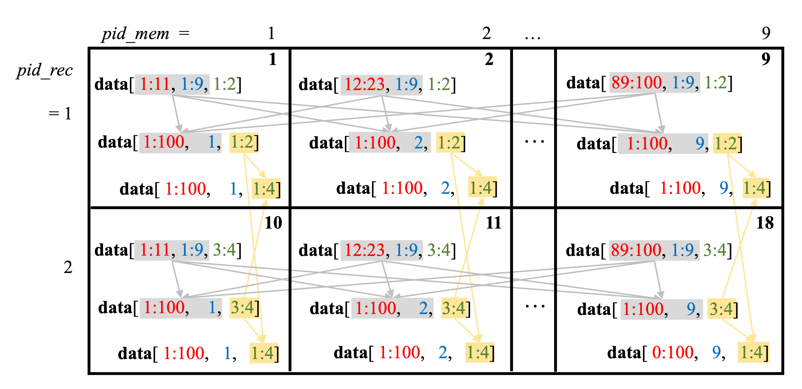
Schematic of the state and observation transpose operations. Gray arrows: state transpose (field-complete fields_prior → ensemble-complete state_prior). Yellow arrows: the additional comm_rec allgather that collects all observation records needed by each processor for the local observation ensembles.

State transpose. State.transpose_to_ensemble_complete(c, fields_prior) communicates within comm_mem to move the field-complete fields_prior (FieldEns) into the ensemble-complete state_prior (StateEns). The same transpose is applied to fields_z to produce state_z. After assimilation, the reverse State.transpose_to_field_complete(c, state_post) brings the ensemble-complete state_post back to field-complete fields_post so that Updator.update(c) can write increments to the model restart files.

Observation transpose. Within each comm_mem record group, only the processor with pid_mem == 0 reads and processes the actual observations via collect_obs_seq(); the result is then broadcast to all other pid_mem in the same group. All pid_mem independently compute observation priors for their own members.

The transpose proceeds in two steps (performed separately for the observation sequence and the observation prior ensemble):

1. Within comm_mem: send the field-complete observations/priors from the source processor to the destination processors so that each processor holds the full ensemble for its own subset of partitions par_list[pid_mem].

2. Across comm_rec: allgather all obs_rec_id within comm_rec so that each pid_rec has the complete set of observation records needed to update its own rec_list.

Concretely, Obs.transpose_obs_seq(c, obs_seq) converts obs_seq (ObsSeq) to lobs (LocalObsSeq), and Obs.transpose_to_ensemble_complete(c, obs_prior) converts obs_prior (ObsEns) to lobs_prior (LocalObsEns). Both are called by Assimilator.transpose_to_ensemble_complete(c).

Assimilation Modes

Once the transposes are complete, each processor holds the local ensemble state_prior[mem_id, rec_id][par_id] (np.ndarray), lobs[obs_rec_id][par_id] (dict[str, np.ndarray]), and lobs_prior[mem_id, obs_rec_id][par_id] (np.ndarray). Before calling the assimilation algorithm, both state and observation data are packed into flat arrays via State.pack_local_state_data(c, par_id, ...) and Obs.pack_local_obs_data(c, par_id, ...).

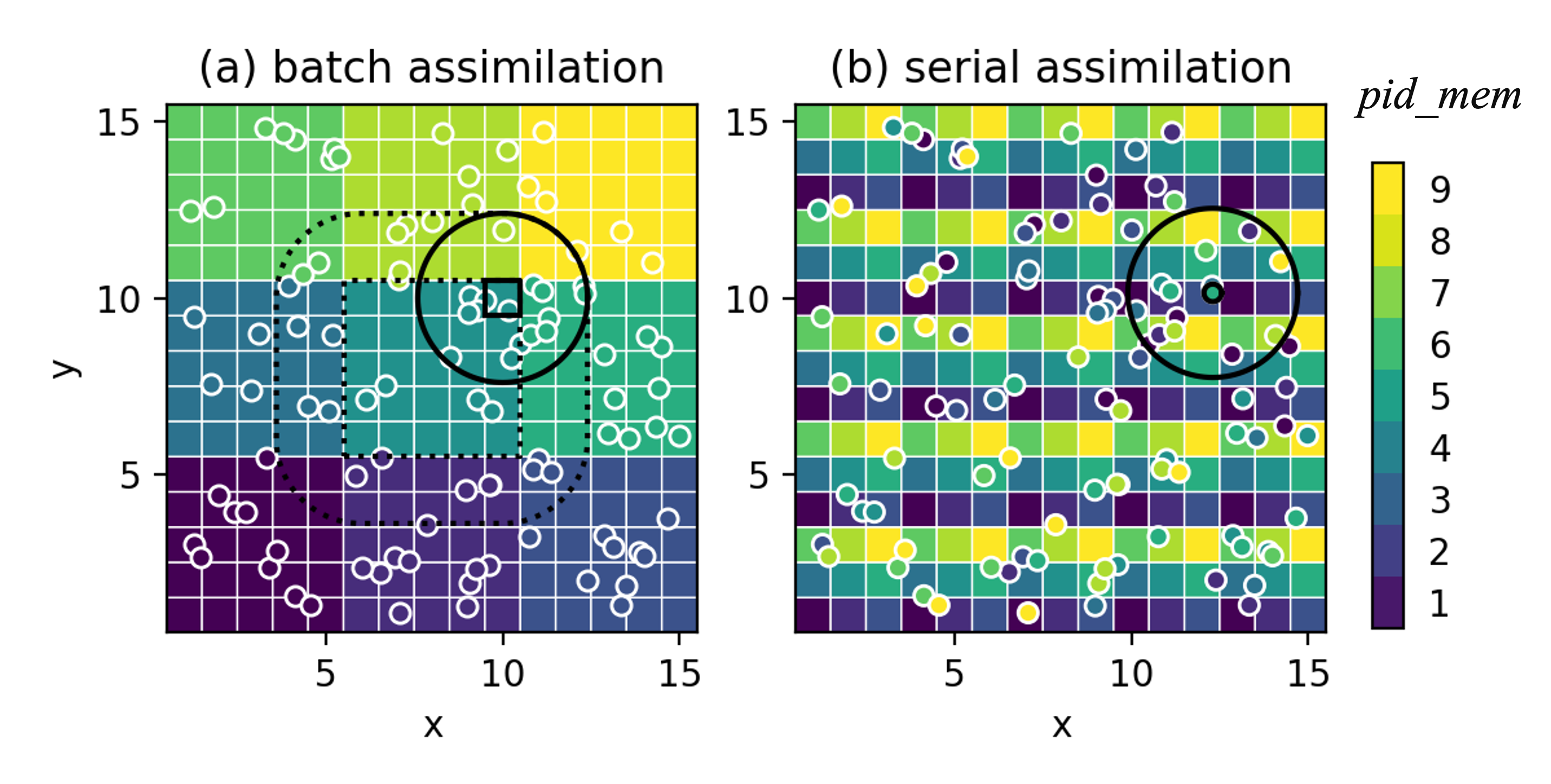
Batch mode (BatchAssimilator).** The analysis domain is divided into square tiles (par_id), with ~3 × nproc_mem tiles to allow load-balanced distribution. BatchAssimilator.assimilation_algorithm(c) loops over par_list[pid_mem]; for each tile it loops over unmasked grid points and calls local_analysis(c, loc_id, ind, hlfactor, state_data, obs_data) with the subset of observations within the horizontal localisation radius hroi. Implemented algorithms include matrix-form ensemble filters such as LETKF and DEnKF. Batch mode is favourable when the local observation volume is small or when the matrix formulation enables more flexible error-covariance modelling.

Serial mode (SerialAssimilator).** Partitions tile the domain so that each pid_mem owns one non-overlapping subset spanning the full domain. SerialAssimilator.assimilation_algorithm(c) iterates over a global ordered list of individual observations. For each observation the owning processor computes obs_increment(obs_prior, obs, obs_err_std) and broadcasts it; all processors then call update_local_state(...) and update_local_obs(...) to update the state and observation priors within the localisation radius. Updated observation priors are reused for subsequent observations, making the update iterative. Serial mode scales better for inhomogeneous networks or large local observation volumes, and scalar updates enable nonlinear filtering approaches such as particle filters or rank regression.

Assimilation Workflow

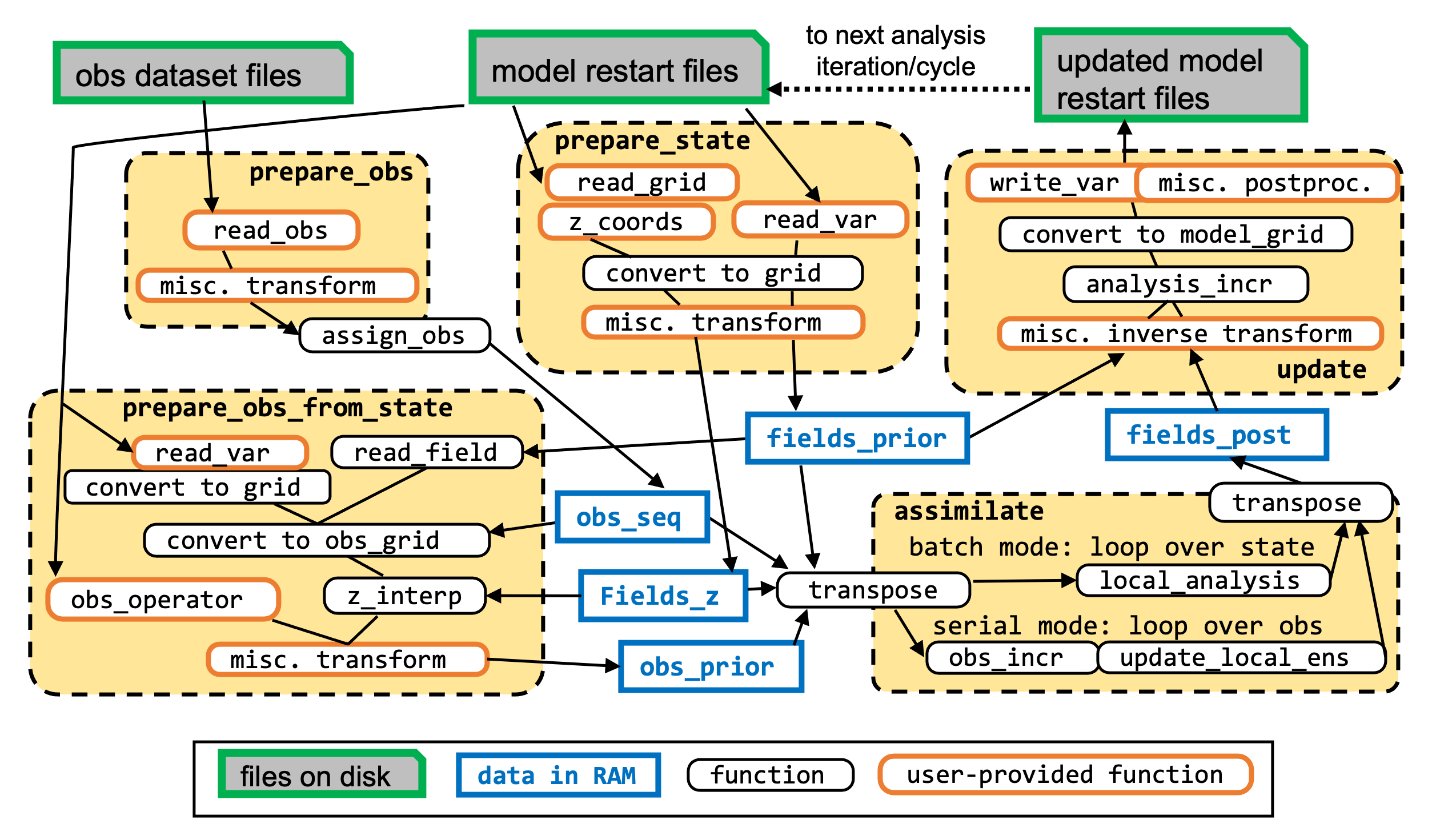
Workflow for one assimilation cycle/iteration. Key variables and functions are shown; black arrows indicate the flow of information. User-provided functions (read_var, z_coords, read_obs, obs_operator) are the interface between model/dataset modules and the core DA algorithms.

Key Variables

Indices and communicators

• pid — rank in the global communicator comm of size nproc.

• pid_mem — rank within comm_mem (record group); pid_mem = pid % nproc_mem.

• pid_rec — rank within comm_rec (member group); pid_rec = pid // nproc_mem.

• comm_mem — sub-communicator grouping all processors with the same pid_rec.

• comm_rec — sub-communicator grouping all processors with the same pid_mem.

• mem_list: dict[ProcIDMem, list[MemID]] — maps each pid_mem to its list of member indices mem_id.

• rec_list: dict[ProcIDRec, list[FieldRecordID]] — maps each pid_rec to its list of field record indices rec_id.

• obs_rec_list: dict[ProcIDRec, list[ObsRecordID]] — maps each pid_rec to its list of observation record indices obs_rec_id.

• partitions: list — spatial partitions of the analysis domain. Each entry is either a slice tuple (istart, iend, di, jstart, jend, dj) (regular 2D grid) or an index array (irregular grid).

• par_list: dict[ProcIDMem, list[PartitionID]] — maps each pid_mem to its list of partition indices par_id.

• obs_inds: dict[ObsRecordID, dict[PartitionID, np.ndarray]] — for each obs_rec_id and par_id, the integer indices into the full observation record that belong to the local observation subset for that partition.

Data structures

• fields_prior: FieldEns — dict[(MemID, FieldRecordID), np.ndarray]. Field-complete prior state; each value is a 2D field fld[j, i] (or fld[2, j, i] for vector fields).

• fields_z: FieldEns — same structure as fields_prior; holds z-coordinate fields for each record.

• state_prior: StateEns — dict[(MemID, FieldRecordID), dict[PartitionID, np.ndarray]]. Ensemble-complete prior state; state_prior[mem_id, rec_id][par_id] is the 1-D array of unmasked field values in the partition.

• state_z: StateEns — same structure as state_prior; holds z-coordinate values in ensemble-complete layout.

• state_post: StateEns — same structure as state_prior; holds the posterior (updated) state after assimilation.

• fields_post: FieldEns — field-complete posterior, produced by transposing state_post back.

• obs_seq: ObsSeq — dict[ObsRecordID, dict[str, np.ndarray]]. Full observation sequence for each record; mandatory keys are 'obs', 'x', 'y', 'z', 't', 'err_std'.

• obs_prior: ObsEns — dict[(MemID, ObsRecordID), np.ndarray]. Observation priors computed from the model state; each value has the same length as obs_seq[obs_rec_id]['obs'].

• lobs: LocalObsSeq — dict[ObsRecordID, dict[PartitionID, dict[str, np.ndarray]]]. Ensemble-complete local observation sequence; lobs[obs_rec_id][par_id] has the same keys as obs_seq but contains only the subset indexed by obs_inds[obs_rec_id][par_id].

• lobs_prior: LocalObsEns — dict[(MemID, ObsRecordID), dict[PartitionID, np.ndarray]]. Ensemble-complete local observation priors; lobs_prior[mem_id, obs_rec_id][par_id] contains the subset of observation priors for that partition.

• lobs_post: LocalObsEns — same structure as lobs_prior; holds the posterior observation ensemble (updated in serial mode only).

Key Functions

• State.prepare_state(c) — for each (mem_id, rec_id) in the local task lists, calls the model module’s read_var() to read variables on the model native grid, converts them to the analysis grid, and applies user-defined transform functions. Also reads z-coordinate fields via z_coords(). Populates fields_prior and fields_z.

• Obs.prepare_obs(c) — calls collect_obs_seq() on the root of each comm_mem group (pid_mem == 0), then broadcasts the result to all other pid_mem in the group. collect_obs_seq() calls the dataset module’s read_obs() for each obs_rec_id in obs_rec_list[pid_rec] and applies transforms. Populates obs_seq.

• Obs.prepare_obs_from_state(c, tag) — for each (mem_id, obs_rec_id) in the local task lists, calls state_to_obs() to compute observation priors from the model state. Three paths are available: (1) read directly from the state if the observed variable is a state variable; (2) call model.read_var() and interpolate horizontally and vertically to the observation network; (3) call a user-provided obs_operator() from the dataset module. Populates obs_prior.

• Assimilator.assign_obs(c) — abstract method implemented differently in each assimilation mode. In batch mode: for each obs_rec_id, finds the observation indices that fall within hroi of each partition bounding box. In serial mode: divides the full observation sequence into nproc_mem non-overlapping subsets, one per par_id. Returns obs_inds: dict[ObsRecordID, dict[PartitionID, np.ndarray]].

• Assimilator.transpose_to_ensemble_complete(c) — orchestrates the full transpose step by calling:

  • State.transpose_to_ensemble_complete(c, fields_prior) → state_prior

  • State.transpose_to_ensemble_complete(c, fields_z) → state_z

  • Obs.transpose_obs_seq(c, obs_seq) → lobs

  • Obs.transpose_to_ensemble_complete(c, obs_prior) → lobs_prior

• BatchAssimilator.assimilation_algorithm(c) — loops over par_list[pid_mem]; for each partition packs state and observation data into flat arrays, then loops over unmasked grid points and calls local_analysis(c, loc_id, ind, hlfactor, state_data, obs_data) to compute the matrix-form local analysis. Writes results to state_post via State.unpack_local_state_data(c, par_id, state_post, state_data).

• SerialAssimilator.assimilation_algorithm(c) — builds a global ordered observation list via Obs.global_obs_list(c), then iterates over individual observations. For each observation: the owning pid_mem calls obs_increment(obs_prior, obs, obs_err_std) and broadcasts the result; all processors call update_local_state(...) and update_local_obs(...) to iteratively update the state and the observation priors in their local partitions.

• Assimilator.transpose_to_field_complete(c) — calls State.transpose_to_field_complete(c, state_post) → fields_post and, in serial mode, Obs.transpose_to_field_complete(c, lobs_post) → obs_post.

• Updator.update(c) — computes analysis increments by calling compute_increment(c) (which compares fields_prior and fields_post), then applies them to the model restart files via update_files(c, mem_id, rec_id) for each (mem_id, rec_id) in the local task lists. User-defined inverse transforms and post-processing steps (e.g. optical-flow alignment) can be inserted in the Updator subclass.

Extensions

The modular design allows the following extensions without changing the core assimilation code:

• Ensemble smoothing — add multiple time steps in the time dimension of the state and/or observations.

• Iterative smoothers — run the analysis cycle as an outer loop (controlled by config.niter).

• Multiscale DA — use spatial bandpass filtering transforms to assimilate each scale component separately (controlled by config.resolution_level).

• Gaussian anamorphosis — apply a transform to map non-Gaussian variables to a Gaussian space before assimilation.

• Nonlinear observation operators — provide a custom obs_operator() in the dataset module to map state to observation space via, e.g., a neural network or radiative transfer model.