Offline filtering analysis scheme

Parallelization strategy

A compromise is made in favor of code flexibility than its runtime efficiency. We aim for more modular design so that components in the DA algorithm can be easily changed/upgraded/compared. A pause-restart strategy is used: the model writes the state to restart files, then DA reads those files and computes the analysis and outputs to the updated files, and the model continues running. This is “offline” assimilation. In operational systems, sometimes we need “online” algorithms where everything is hold in the memory to avoid slow file I/O. NEDAS provides parallel file I/O, not suitable for time-critical applications, but efficient enough for most research and development purposes.

The first challenge on dimensionality demands a careful design of memory layout among processors. The ensemble model state has dimensions: member, variable, time, z, y, x. When preparing the state, it is easier for a processor to obtain all the state variables for one member, since they are typically stored in the same model restart file. Each processor can hold a subset of the ensemble states, this memory layout is called “state-complete”. To apply the ensemble DA algorithms, we need to transpose the memory layout to “ensemble-complete”, where each processor holds the entire ensemble but only for part of the state variables (Anderson & Collins 2007).

In NEDAS, for each member the model state is further divided into “fields” with dimensions (y, x) and “records” with dimensions (variable, time, z). Because, as the model dimension grows, even the entire state for one member maybe too big for one processor to hold in its memory. The smallest unit is now the 2D field, and each processor holds only a subset along the record dimension. Accordingly, the processors (pid) are divided into “member groups” (with same pid_rec) and “record groups” (with same pid_mem), see Fig. 1 for example. “State-complete” now becomes “field-complete”. The record dimension allows parallel processing of different fields by the read_var functions in model modules. And during assimilation, each pid_rec only solves the analysis for its own list of rec_id.

figure ../imgs/transpose.png

Transpose from field-complete to ensemble-complete, illustrated by a 18-processor memory layout (pid = 1, …, 18), divided into 2 groups (pid_rec = 0, 1), each with 9 processors (pid_mem = 0, 1, 2). The data has dimensions mem_id = 1:100 members, par_id = 1:9 partitions, and rec_id = 1:4 records. The gray arrows show sending/receiving of data to perform the transpose. The yellow arrows is an additional collection step (only needed by observation data)

For observations, it is easier to process the entire observing network at once, instead of going through the measurements one by one. Therefore, each observing network (record) is assigned a unique obs_rec_id to be handled by one processor. Each pid_rec only needs to process its own list of obs_rec_id. Processors with pid_mem = 0 is responsible for reading and processing the actual observations using read_obs functions from dataset modules, while all pid_mem separately process their own members for the observation priors. When transposing from field-complete to ensemble-complete is done, an additional collection step among different pid_rec is required, which gathers all obs_rec_id for each rec_id to form the final local observation.

When the transpose is complete, on each pid, the local ensemble state_prior[mem_id, rec_id][par_id] is updated to the posterior state_post, using local observations lobs[obs_rec_id][par_id] and observation priors lobs_prior[mem_id, obs_rec_id][par_id].

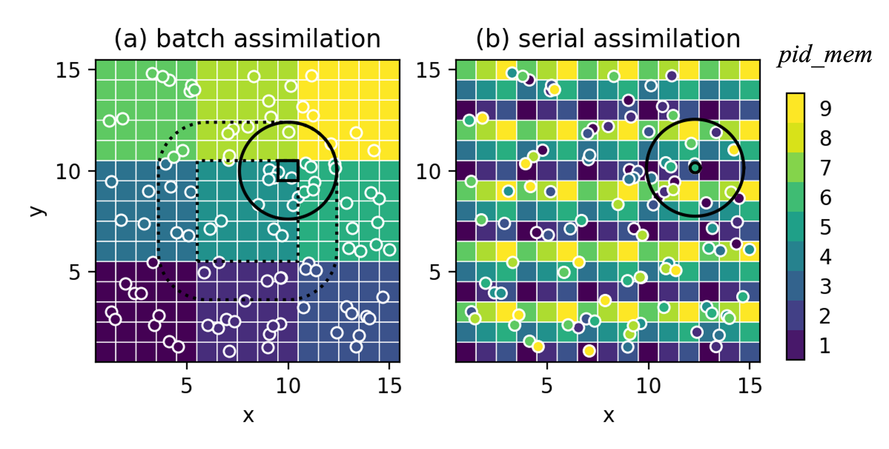
Memory layout for state variables (square pixels) and observations (circles) using (a) batch and (b) serial assimilation strategies. The colors represent the processor id pid_mem that stores the data.

NEDAS offline filter scheme provides two assimilation modes:

In batch mode, the analysis domain is divided into small local partitions (indexed by par_id) and each pid_mem solves the analysis for its own list of par_id. The local observations are those falling inside the localization radius for each [par_id,`rec_id`]. The “local analysis” for each state variable is computed using the matrix-version ensemble filtering equations (such as [LETKF](https://doi.org/10.1016/j.physd.2006.11.008), [DEnKF](https://doi.org/10.1111/j.1600-0870.2007.00299.x)). The batch mode is favorable when the local observation volume is small and the matrix solution allows more flexible error covariance modeling (e.g., to include correlations in observation errors).

In serial mode, we go through the observation sequence and assimilation one observation at a time. Each pid stores a subset of state variables and observations with par_id, here locality doesn’t matter in storage, the pid owning the observation being assimilated will first compute observation-space increments, then broadcast them to all the pid with state_prior and/or lobs_prior within the observation’s localization radius and they will be updated. For the next observation, the updated observation priors will be used for computing increments. The whole process iteratively updates the state variables on each pid. The serial mode is more scalable especially for inhomogeneous network where load balancing is difficult, or when local observation volume is large. The scalar update equations allow more flexible use of nonlinear filtering approaches (such as particle filter, rank regression).

NEDAS allows flexible modifications in the interface between model/dataset modules and the core assimilation algorithms, to achieve more sophisticated functionality:

Multiple time steps can be added in the time dimension for the state and/or observations to achieve ensemble smoothing instead of filtering. Iterative smoothers can also be formulated by running the analysis cycle as an outer-loop iteration (although they can be very costly).

Miscellaneous transform functions can be added for state and/or observations, for example, Gaussian anamorphosis to deal with non-Gaussian variables; spatial bandpass filtering to run assimilation for “scale components” in multiscale DA; neural networks to provide a nonlinear mapping between the state space and observation space, etc.

Description of Key Variables and Functions

`{figure} ../imgs/workflow.png :width: 100% :align: center ` <!–| Figure 3. Workflow for one assimilation cycle/iteration. For the sake of clarity, only the key variables and functions are shown. Black arrows show the flow of information through functions.| –>

Indices and lists:

• For each processor, its pid is the rank in the communicator comm with size nproc. The comm is split into comm_mem and comm_rec. Processors in comm_mem belongs to the same record group, with pid_mem in [0:nproc_mem]. Processors in comm_rec belongs to the same member group, with pid_rec in [0:nproc_rec]. Note that nproc = nproc_mem * nproc_rec, user should set nproc and nproc_mem in the config file.

• mem_list`[`pid_mem] is a list of members mem_id for processors with pid_mem to handle.

• rec_list`[`pid_rec] is a list of field records rec_id for processors with pid_rec to handle.

• obs_rec_list`[`pid_rec] is a list of observation records obs_rec_id for processors with pid_rec to handle.

• partitions is a list of tuples (istart, iend, di, jstart, jend, dj) defining the partitions of the 2D analysis domain, each partition holds a slice [istart:iend:di, jstart:jend:dj] of the field and is indexed by par_id.

• par_list`[`pid_mem] is a list of partition id par_id for processor with pid_mem to handle.

• obs_inds`[`obs_rec_id][par_id] is the indices in the entire observation record obs_rec_id that belong to the local observation sequence for partition par_id.

Data structures:

• fields_prior`[`mem_id, rec_id] points to the 2D fields fld[…] (np.array).

• z_fields`[`mem_id, rec_id] points to the z coordinate fields z[…] (np.array).

• state_prior`[`mem_id, rec_id][par_id] points to the field chunk fld_chk (np.array) in the partition.

• obs_seq`[`obs_rec_id] points to observation sequence seq that is a dictionary with keys (‘obs’, ‘t’, ‘z’, ‘y’, ‘x’, ‘err_std’) each pointing to a list containing the entire record.

• lobs`[`obs_rec_id][par_id] points to local observation sequence lobs_seq that is a dictionary with same keys as seq but the lists only contain a subset of the record.

• obs_prior_seq`[`mem_id, obs_rec_id] points to the observation prior sequence (np.array), same length with seq[‘obs’].

• lobs_prior`[`mem_id, obs_rec_id][par_id] points to the local observation prior sequence (np.array), same length with lobs_seq.

Functions:

• prepare_state(): For member mem_id in mem_list and field record rec_id in rec_list, load the model module and read_var() gets the variables in model native grid, convert to analysis grid, and apply miscellaneous user-defined transforms. Also, get z coordinates in the same prodcedure using z_coords() functions. Returns fields_prior and z_fields.

• prepare_obs(): For observation record obs_rec_id in obs_rec_list, load the dataset module and read_obs() get the observation sequence. Apply miscellaneous user-defined transforms if necessary. Returns obs_seq.

• assign_obs(): According to (‘y’, ‘x’) coordinates for par_id and (‘variable’, ‘time’, ‘z’) for rec_id, sort the full observation sequence obs_rec_id to find the indices that belongs to the local observation subset. Returns obs_inds.

• prepare_obs_from_state(): For member mem_id in mem_list and observation record obs_rec_id in obs_rec_list, compute the observation priors from model state. There are three ways to get the observation priors: 1) if the observed variable is one of the state variables, just get the variable with read_field(), or 2) if the observed variable can be provided by model module, then get it through read_var() and convert to analysis grid. These two options obtains observed variables defined on the analysis grid, then we convert them to the observing network and interpolate to the observed z location. Option 3) if the observation is a complex function of the state, the user can provide obs_operator() in the dataset module to compute the observation priors. Finally, the same miscellaneous user-defined transforms can be applied. Returns obs_prior_seq.

• transpose_field_to_state(): Transposes field-complete field_prior to ensemble-complete state_prior (illustrated in Fig.1). After assimilation, the reverse transpose_state_to_field() transposes state_post back to field-complete fields_post.

• transpose_obs_to_lobs(): Transpose the obs_seq and obs_prior_seq to their ensemble-complete counterparts lobs and lobs_prior (illustrated in Fig. 2).

• batch_assim(): Loop through the local state variables in state_prior, for each state variable, the local observation sequence is sorted based on the localization and impact factors. If the local observation sequence is not empty, compute the local_analysis() to update state variables, save to state_post and return.

• serial_assim(): Loop through the observation sequence, for each observation, the processor storing this observation will compute obs_increment() and broadcast. For all processors, if some of its local state/observations are within the localization radius of this observation, compute update_local_ens() to update these state/observations. Do this iteratively for all observations until end of sequence. Returns the updated local state_post.

• update(): Take state_prior and state_post, apply miscellaneous user-defined inverse transforms, compute analysis_incr(), convert the increment back to model native grid and add the increments to the model variables int he restart files. Apart from simply adding the increments, some other post-processing steps can be implemented, for example using the increments to compute optical flows and align the model variables instead.

NEDAS.schemes.filter module

class NEDAS.schemes.filter.FilterAnalysisScheme(config: Config | None = None, config_file: str | None = None, parse_args: bool = False, **kwargs)

Bases: Scheme

Scheme subclass for performing filter analysis.

This scheme runs the 4D analysis by cycling through time steps. Running the ensemble forecast first, pause the model at a certain time step (analysis cycle), then perform data assimilation at the analysis cycle with observations within a time window, finally using the updated model states (the posterior) as new initial conditions, the ensemble forecast is run again to reach the next analysis cycle, until the end of the period of interest. The length of forecasts between cycles is called the cycling period.

steps_need_mpi: dict[str, bool] = {'diagnose': True, 'ensemble_forecast': False, 'filter': True, 'perturb': True, 'postprocess': False, 'prepare_init_ensemble': False, 'prepare_truth': False, 'preprocess': False, 'run_all': True}

run_all() → None

A schemem must implement a run_all method to describe the workflow.

load_model_state(time: datetime)

save_model_state(time: datetime)

load_obs(time: datetime)

save_obs(time: datetime)

prepare_truth() → None

Generate the verifying truth

validate_truth_data(model_name: str) → bool

prepare_init_ensemble() → None

Generate initial ensemble.

validate_init_ensemble_data(model_name)

check_cycle_complete() → bool

Method checks on a given cycle to see if it’s complete or not

preprocess() → None

Pre-processing step before the assimilation.

postprocess() → None

Post-processing step after the assimilation and before the next forecast.

ensemble_forecast() → None

Ensemble forecast step.

filter() → None

Main method for performing the analysis step

filter_iter() → None

perturb() → None

Perturbation step.

This step adds random perturbations to the model initial and/or boundary conditions, at the first or all the analysis cycles.

diagnose() → None

Diagnostics step.

This step runs diagnostics for the current analysis cycle.

The diag section in configuration file defines the methods and parameters of the diagnostics, corresponding to the diag.method module that implements the particular diagnostic method.

get_task_opts(step: str, model_name: str, **other_opts) → dict[str, Any]

Get common kwargs from configuration and return as task options dict

get_restart_dir(model_name) → str

NEDAS.schemes.filter.main()